Thanksgiving Night Build: Dual ITR1204 IR Sensor Test Module
The house got quiet on Thanksgiving night, so I opened KiCad and finally started the encoder board that’s been sitting in my backlog. It’s a $0.60, dual-channel reflective IR sensor that’s the first step toward closing the loop on cheap servos.
If you’re new here, OpenServoCore is my effort to turn cheap MG90S-class servos into networked smart actuators with sensor feedback, cascade control, and a DYNAMIXEL-style TTL bus. To get there I need a reliable, low-cost way to measure motor motion, and this board is Part 1 of that. It’s a tiny ITR1204-based PCB that handles the detection stage. Part 2 will be the MCU and comparator front-end once these come back from fab.
In this post you’ll find the schematic and 4-layer layout, a full walk through four operating modes (5 V and 3.3 V, digital and analog) with the math behind each resistor pair, a BOM that lands at roughly $0.60 per board, and JLCPCB ordering notes for both bare-PCB and full PCBA paths. The board is intentionally retunable by swapping two resistor pairs, so the same footprint works as a quadrature edge sensor or a direct-to-ADC analog encoder.
So without further ado, let’s dive into the details of this board.
More info:
TL;DR
- Built a compact dual-channel IR reflective sensor board using ITR1204SR10A_TR(BY).
- As-populated, it runs in 5 V “digital” mode: ~9–10 mA LED current, fast edges + small ~0–0.2 V analog deltas meant for an external MCU + comparator/op-amp board.
- By swapping only two resistor pairs (LED current-limit + pull-down), the same PCB can be configured in four modes:
- 5 V digital - 390 Ω LED, 680 Ω pull-down (current build)
- 3.3 V digital - 220 Ω LED, 680 Ω pull-down
- 5 V analog (ADC) - 390 Ω LED, 15 kΩ pull-down
- 3.3 V analog (ADC) - 220 Ω LED, 10 kΩ pull-down
- Secondary goal: experiment with pure analog encoder approaches for angular position, going straight into an MCU ADC or Schmitt-trigger GPIO with minimal BOM.
- Intended for evaluating reflective sensing robustness before committing to a tight internal servo encoder.
Render / Photo
Why this board exists
OpenServoCore needs a reliable way to measure motor speed and dynamic response during system identification and early control development.
This board exists to:
A) Serve as an external system identification sensor
- Mount over a patterned disk or strip
- Produce stable A/B signals
- Feed into an amplifier/comparator
- Capture accurate speed traces for system modeling
B) Prototype a future integrated encoder
Before designing a flex-PCB encoder under the gearbox inside a servo (extremely tight space), I need to:
- Characterize distances
- Optimize LED current
- Understand real-world reflectivity
- Measure output deltas
- Determine if a minimal BOM analog angle encoder is feasible
This board is the platform for exploring both.
Schematic
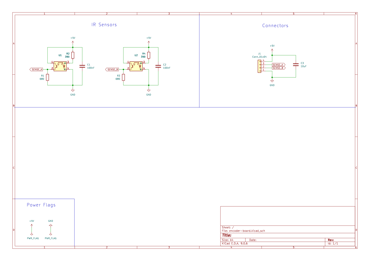
Circuit Overview
Sensors:
- U1, U2: ITR1204SR10A_TR(BY) reflective IR pairs (LCSC: C475373)
LED current-limit resistors:
- R2, R4 = 390 Ω (IR LEDs)
Phototransistor pull-downs:
- R1, R3 = 680 Ω
Filtering:
- C1, C2 = 100 nF local decoupling
- C3 = 10 µF bulk decoupling
Connector:
- J1: 4-pin header (GND, B, A, 5V)
The output signals are low-level analog, not cleaned or thresholded, and this is intentional.
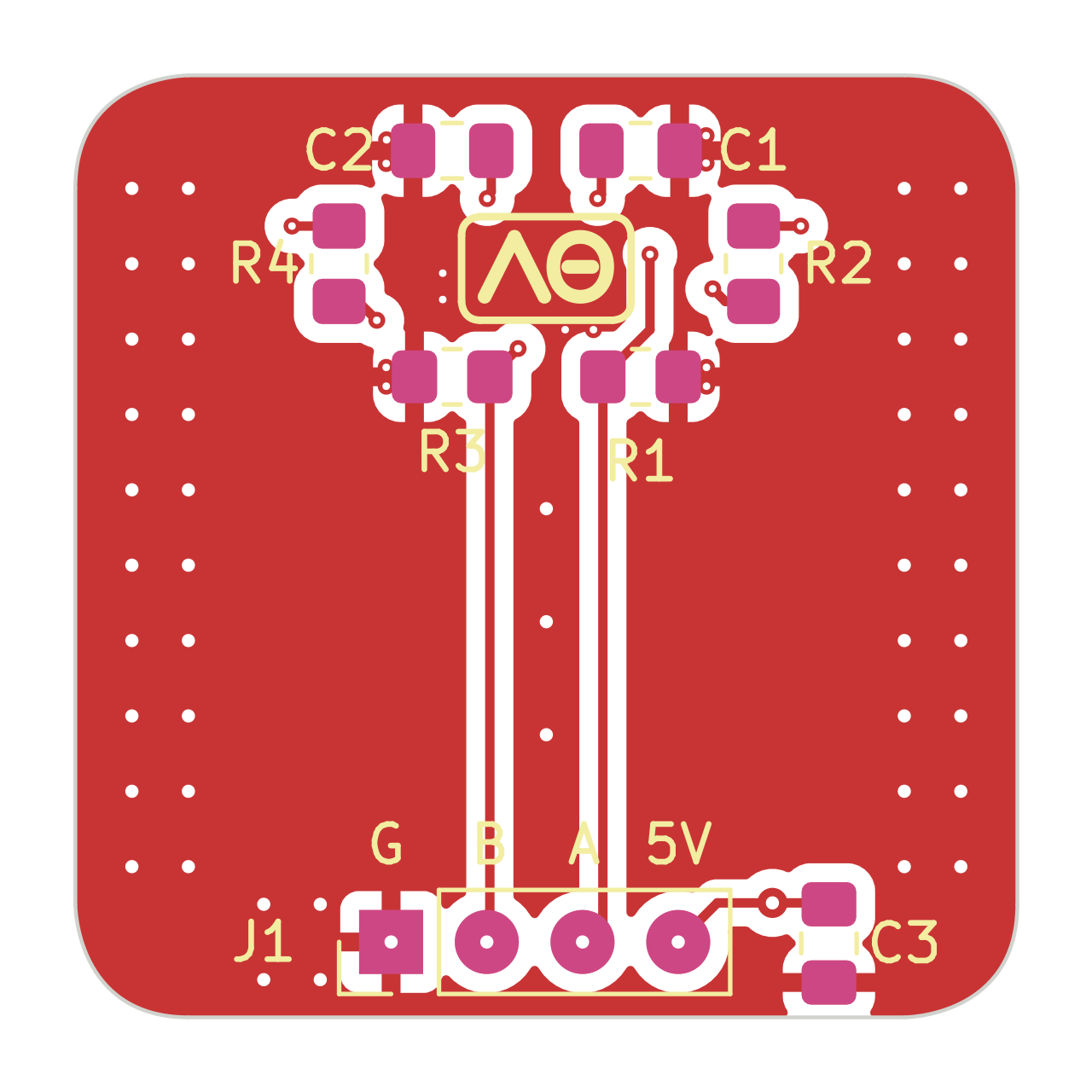
PCB Layout
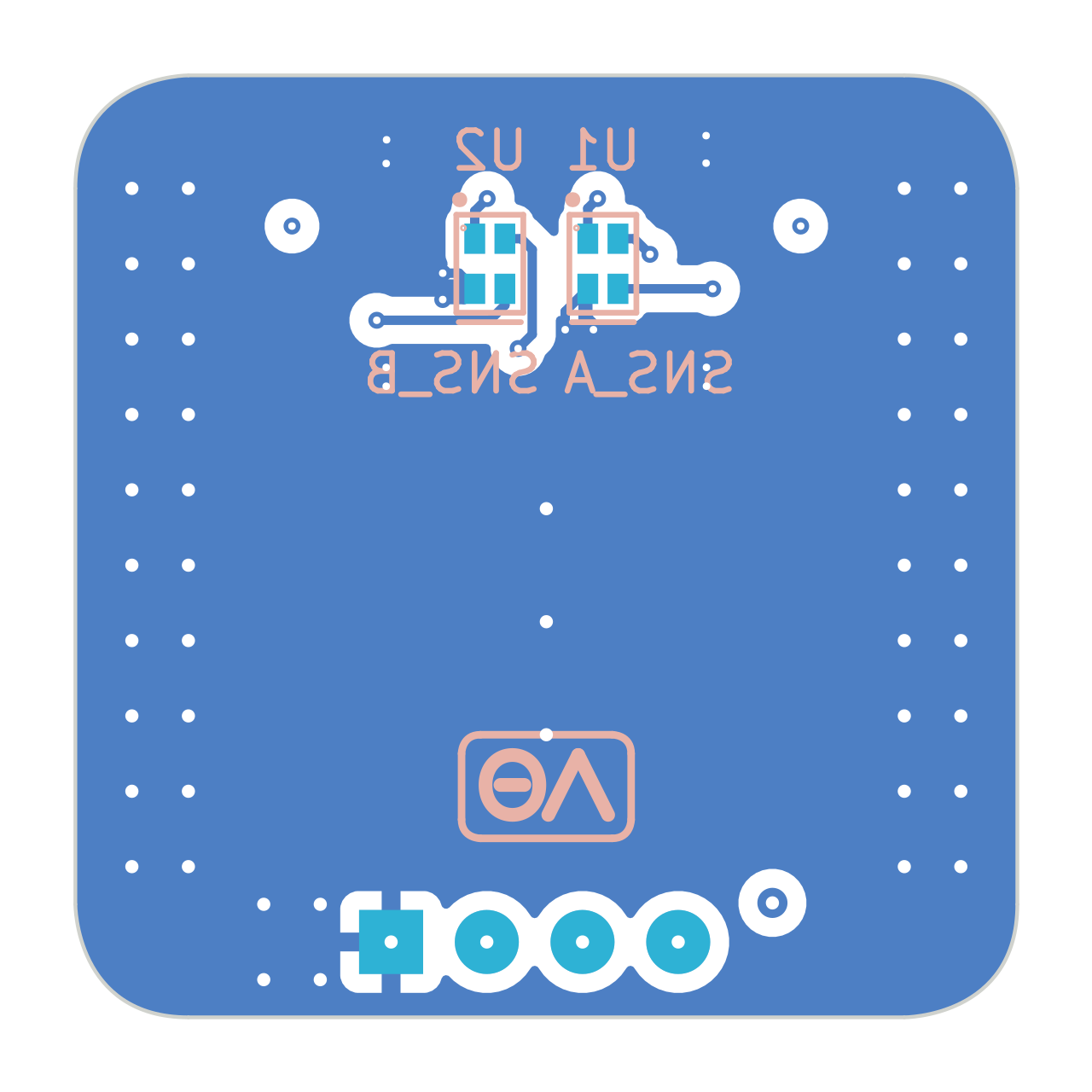
This is a 4-layer board. The inner layers are dedicated VCC and GND planes for clean power and low-impedance return paths. Around the two IR sensors there’s a small exclusion zone in the VCC plane so the active area sees less capacitive coupling and noise from the supply copper directly under the sensing region.
All the passives and the connector live on the front. The sensors sit alone on the back so this face can be pushed right up against an encoder disk or tucked inside a shroud.
All resistors and capacitors are 0805 with generous hand-solder footprints. That’s intentional, this board is meant to be easy to retune by swapping R values as you experiment with 5 V vs 3.3 V, digital vs analog, or different LED currents and pull-downs.
Operating modes & resistor selection
This board is intentionally simple enough that you can “retune” it just by changing resistor values.
All four modes below use the same datasheet numbers for ITR1204SR10A_TR(BY) :
- Forward voltage: VF ≈ 1.25 V typ, 1.5 V max @ IF = 4 mA
- Reflective “on” current: IC(ON) ≈ 70–130 µA @ IF = 4 mA, VCE = 2 V, RL = 1 kΩ
- Rise/fall time: tr, tf ≈ 15 µs @ RL = 1 kΩ
When we push the LED harder (≈ 9–10 mA) we scale IC(ON) roughly by ~2.3–2.5×:
- IF ≈ 9–10 mA → IC(ON) ≈ 160–320 µA (rule-of-thumb)
Everything below assumes that range.
1. 5 V “digital” mode (current board)
Goal: Fast edges, low impedance, small ~0–0.2 V swing that you clean up with an external op-amp / comparator.
Resistor values (as-built):
- R_LED (R2, R4) = 390 Ω
- R_PD (R1, R3) = 680 Ω
LED current @ 5 V
Using:
$$ I_{LED} = \frac{V_{CC} - V_F}{R} $$At VF = 1.25 V:
$$ I_{LED} \approx \frac{5 - 1.25}{390} \approx 9.6\ \text{mA} $$At VF = 1.5 V:
$$ I_{LED} \approx \frac{5 - 1.5}{390} \approx 9.0\ \text{mA} $$
So we’re safely at ~9–10 mA, about 2.2–2.5× the datasheet’s 4 mA test current.
Phototransistor output swing @ 5 V
We approximate:
$$ I_C \approx 160–320\ \mu\text{A} $$With R_PD = 680 Ω:
$$ V_{OUT} = I_C \cdot R_{PD} $$- At 160 µA → ≈ 0.11 V
- At 220 µA (nice “typical” mid-point) → ≈ 0.15 V
- At 320 µA → ≈ 0.22 V
So you get ~0–0.2 V low-level analog deltas.
Why this works well for comparators
- Low impedance (680 Ω) keeps edges sharp and limits cable / input capacitance effects.
- You’re well below the 1 kΩ used in the datasheet’s 15 µs rise/fall spec, so real edges will be at least as fast.
- Comparator on the next board can set whatever threshold/hysteresis it wants. This board just has to deliver clean, small deltas near ground.
This is exactly the mode described in the rest of this log.
2. 3.3 V “digital” mode
Goal: Same behavior as the 5 V digital mode (fast edges, ~0–0.2 V swing), but powered from 3.3 V and intended to feed a 3.3 V comparator / MCU front-end.
We keep the same phototransistor behavior (same IC range), and just retune the LED resistor so that LED current stays in the same 9–10 mA ballpark.
Resistor values (3.3 V digital):
- R_LED (R2, R4) = 220 Ω (instead of 390 Ω)
- R_PD (R1, R3) = 680 Ω (same as 5 V digital)
LED current @ 3.3 V
$$ I_{LED} = \frac{V_{CC} - V_F}{R} $$Using VF = 1.25–1.5 V:
At VF = 1.25 V:
$$ I_{LED} \approx \frac{3.3 - 1.25}{220} \approx 9.3\ \text{mA} $$At VF = 1.5 V:
$$ I_{LED} \approx \frac{3.3 - 1.5}{220} \approx 8.2\ \text{mA} $$
So LED current is very close to the 5 V digital case, which means:
- similar reflected photocurrent (IC(ON))
- similar usable distance (~2 mm region)
- similar noise margin into your comparator
Phototransistor swing @ 3.3 V
The collector current is set by optics, not by VCC, so we keep the same 160–320 µA estimate. With R_PD = 680 Ω, the math is identical:
- 160 µA → ≈ 0.11 V
- 220 µA → ≈ 0.15 V
- 320 µA → ≈ 0.22 V
That tiny swing is still well within the input common-mode range of 3.3 V rail-to-rail op-amps / comparators, and low impedance keeps edges fast.
In other words, for 3.3 V digital use, just change the LED resistors to 220 Ω and leave everything else alone.
3. 5 V “analog” mode (direct ADC)
Goal: Use the sensor as a fine-grained analog position tap, feeding an ADC (or possibly a Schmitt-trigger GPIO). Instead of timing edges for RPM, this mode prioritizes a larger, more linear voltage swing vs. angle so you can resolve small changes in shaft position.
We keep the same LED current (and therefore similar optical behavior) and just increase the pull-down resistor so the output sits high in the ADC range.
Resistor values (5 V analog):
- R_LED (R2, R4) = 390 Ω (same as 5 V digital)
- R_PD (R1, R3) = 15 kΩ (instead of 680 Ω)
Expected swing
Using the same IC ≈ 160–320 µA estimate:
$$ V_{OUT} = I_C \cdot R_{PD} $$For R_PD = 15 kΩ:
- 160 µA → 2.4 V
- 220 µA → 3.3 V
- 320 µA → 4.8 V (in practice this will clip near VCC − V_CE(sat), so expect ≈ 4.6–4.8 V at strong reflection)
So around the “typical” operating point you get roughly 2.4–3.3 V, and for very strong reflections you ride close to the top rail.
For a 5 V ADC, that’s approximately:
- weaker reflection ~2.4 V → ~48% of full-scale
- typical ~3.3 V → ~66% of full-scale
- strong reflection ~4.7 V → >90% of full-scale
Plenty of headroom and a nice, wide usable band near the top of the ADC range.
Trade-offs
- Larger R means slower edges vs the 680 Ω case, but in this analog mode we care more about a stable level vs. angle than about sharp edges for RPM counting. For typical servo joints, the mechanical bandwidth is low enough that this RC penalty is a non-issue.
- The output impedance is now on the order of 15 kΩ, which is still fine for many MCU ADCs if you give them enough sampling time. If your MCU wants a lower source impedance, you can either:
- buffer with a small op-amp, or
- drop R_PD into the 6.8–10 kΩ range and accept a bit less swing.
4. 3.3 V “analog” mode (direct ADC)
Goal: Same idea as the 5 V analog mode. Treat the sensor as a continuous analog encoder for shaft angle, just scaled for a 3.3 V ADC instead of 5 V. The focus is on usable voltage range and repeatability over angle, not on high-speed edge timing.
Again, we reuse the same LED current trick as the 3.3 V digital mode and choose a pull-down that pushes the signal high in the 3.3 V range.
Resistor values (3.3 V analog):
- R_LED (R2, R4) = 220 Ω (same as 3.3 V digital)
- R_PD (R1, R3) = 10 kΩ
LED current @ 3.3 V
Same math as before for 220 Ω:
- ≈ 8.2–9.3 mA → similar IC range (≈ 160–320 µA)
Expected swing into a 3.3 V ADC
With R_PD = 10 kΩ:
$$ V_{OUT} = I_C \cdot R_{PD} $$- 160 µA → 1.6 V
- 220 µA → 2.2 V
- 320 µA → 3.2 V (again, in practice this will clip slightly below VCC due to saturation, expect ≈ 3.0–3.1 V at strong reflection)
For a 3.3 V ADC, that’s roughly:
- weaker reflection ~1.6 V → ~48% of full-scale
- typical ~2.2 V → ~67% of full-scale
- strong reflection ~3.1 V → >90% of full-scale
So the useful analog band again lives in the upper half of the ADC range, with headroom to track contrast changes and calibration.
If you want a larger fraction of the range and don’t mind even higher source impedance (and more saturation at the top), you can:
- push R_PD toward 15 kΩ (mirroring the 5 V case), or
- add a gain/offset stage on a separate analog board and keep R_PD lower.
Summary: which Rs to change
For this PCB, everything stays the same except R2, R4 (LED) and R1, R3 (pull-downs):
| Mode | VCC | R_LED (R2, R4) | R_PD (R1, R3) |
|---|---|---|---|
| 5 V digital | 5 V | 390 Ω | 680 Ω |
| 3.3 V digital | 3.3 V | 220 Ω | 680 Ω |
| 5 V analog | 5 V | 390 Ω | 15 kΩ |
| 3.3 V analog | 3.3 V | 220 Ω | 10 kΩ |
The footprint and BOM entries stay the same, just with different values. Pick the row that matches your system voltage and “digital vs analog” preference, and stuff those resistors accordingly.
Intended use of A/B channels
- A and B are placed with a small spatial offset
- When read over a multi-mark encoder disk, you get “quadrature-ish” signals:
- A leads B in one direction
- B leads A in the reverse direction
These are not digital quadrature signals yet. They are analog reflectivity deltas to be cleaned externally.
Secondary goal: analog-only encoder path
A future experiment (not main goal for this revision):
- Use larger pull-down resistors (≈ 10–15 kΩ for full-range angle sensing)
- Tune LED current + distance
- Feed output directly into MCU ADC or possibly Schmitt-trigger GPIO
- Aim for a minimal-BOM encoder (sensor + 2 resistors)
- Useful for ultra-tight servo integration where no op-amp fits
This revision provides the raw data needed to evaluate feasibility.
BOM (from JLCPCB BOM CSV)
| Value | Designators | LCSC | Qty |
|---|---|---|---|
| 100nF | C1, C2 | C28233 | 2 |
| 10uF | C3 | C15850 | 1 |
| 390 Ω | R2, R4 | C17655 | 2 |
| 680 Ω | R1, R3 | C17798 | 2 |
| Conn_01x04 | J1 | C2905435 | 1 |
| ITR1204SR10A_TR(BY) | U1, U2 | C475373 | 2 |
Approx BOM cost (LCSC small quantity): ~$0.60 per board.
Folder structure (from repo)
hardware/encoder-board/
  └─ jlcpcb/
       ├─ production-files/
       ├─ GERBER-encoder-board.zip
       ├─ BOM-encoder-board.csv
       └─ CPL-encoder-board.csv
Ordering from JLCPCB
Option A - Bare PCB (recommended for prototyping)
If you already have the components, you can skip the assembly process and hand-solder yourself. This only cost me about $6 including shipping for a small batch.
If you’re just getting into SMD, you can also grab 0805 SMD sample books from AliExpress (resistor and capacitor books are usually sold separately). They’re compact, easy to store, and give you a huge spread of R/C values on tap, perfect for boards like this where you might retune resistor values a few times.
For the two IR sensors, hand-soldering is technically possible but not very fun. A small hot plate / mini reflow plate makes life much easier:
- stencil or dab on paste for the sensors
- place them with tweezers
- heat on the plate until reflow
- then hand-solder the 0805 parts and connector
- Upload
GERBER-encoder-board.zip. - Select:
- 1.6 mm PCB, 1 oz copper
- Any solder mask color
- Order a set of 5 or 10.
- Buy components from LCSC (using LCSC codes above) or pull from your 0805 sample books / AliExpress kits.
- Reflow the sensors on a small hot plate, then hand-solder the remaining passives and connector (0805s are very chill with flux and tweezers).
Option B - Full PCBA
- Start SMT Assembly order.
- Upload
GERBER-encoder-board.zip. - Add BOM + CPL files (
BOM-encoder-board.csvandCPL-encoder-board.csv). - (Optional but recommended) Exclude the 1×4 pin header (J1) from assembly to save a bit of cost. Through-hole connectors add a couple of dollars to the PCBA bill, and it’s easy to solder your own header or wires later.
- Carefully review the rotation and side for U1 and U2. I have not run a JLC-assembled batch yet, so please double-check the footprints and orientation in the JLC preview before confirming.
- Confirm top/bottom placement.
- Place the order.
Because the design is simple, assembly is cheap, and skipping the connector keeps it even cheaper.
How to use the board
Reflective IR sensors work by firing IR light at a surface and measuring how much comes back:
- Light / reflective areas (white paper, glossy label, shiny metal, etc.) bounce IR back into the phototransistor → output goes “more on”.
- Dark / non-reflective areas (matte black paint, black tape, printed black toner) reflect very little → output goes “more off”.
By alternating reflective and dark segments on a disk or strip, you turn motion into a changing analog signal. With two sensors (A/B) offset in space, those patterns become “quadrature-ish”. A and B move in and out of the bright/dark zones at slightly different times as the disk moves.
For basic tests:
- Supply +5 V or 3.3 V to J1, depending on which mode you stuffed (see the operating modes table above for resistor values and voltage).
- Connect outputs A/B to a scope or logic analyzer via a simple front-end:
- directly for analog/ADC mode
- or via an external comparator/op-amp board for digital edges.
- Make a simple test target:
- Easiest path: design a black/white striped encoder disk (or strip), print it on a laser printer, cut it out, and glue it onto a 3D-printed disk or any flat plastic hub.
- White paper + black toner works surprisingly well as “reflective vs dark”.
- Mount the sensor board so the back side (with the two IR parts) faces the pattern at ~1–2 mm distance. Adjust the distance until you get good contrast between bright and dark zones.
- Add a simple shroud between the board and the target if possible:
- a 3D-printed or laser-cut U-shaped piece
- painted matte black inside
- walls between A and B to reduce cross-talk (one sensor seeing the other’s LED) and ambient light leakage.
- Sweep the disk/strip slowly by hand:
- In the “digital” resistor configurations, the board still outputs small analog deltas near ground. On a scope you’ll see little bumps as each stripe passes. Once you feed those into a comparator board, you’ll get clean low/high transitions on A and B, offset in time.
- In analog/ADC mode, you’ll see smooth voltage curves as each mark passes under the sensor. A and B curves will be phase-shifted and can be used as an analog encoder for angle.
- For external digital cleanup, feed A/B into an op-amp/comparator front-end and set thresholds + hysteresis so “reflective vs dark” becomes clean logic-level quadrature signals.
- For angle experiments, log the ADC values vs. mechanical position and use that curve as your analog encoder transfer function.
Once you have a pattern that gives good contrast, distance, and minimal cross-talk with a shroud, you can start shrinking the geometry and thinking about how to tuck something similar inside a servo.
Next steps
- Build the MCU + comparator front-end board.
- Log oscilloscope traces at distances 1.0 / 1.5 / 2.0 / 2.5 mm.
- Tune comparator thresholds and hysteresis.
- Experiment with larger pull-down resistors for analog-only encoder path.
- Evaluate feasibility of integrating a miniaturized version inside future OpenServoCore servo housings.